
pandas
needs no introduction as it became the de facto tool for data analysis
in Python. As a Data Scientist, I use pandas daily and I am always
amazed by how many functionalities it has. In this post, I am going to
show you 5 pandas tricks that I learned recently and using them helps me
to be more productive.
For pandas newbies — Pandas
provides high-performance, easy-to-use data structures and data
analysis tools for the Python programming language. The name is derived
from the term “panel data”, an econometrics term for data sets that
include observations over multiple time periods for the same
individuals.
To run the examples download this Jupyter notebook.
To Step Up Your Pandas Game, read:
- 5 lesser-known pandas tricks
- Exploratory Data Analysis with pandas
- How NOT to write pandas code
- 5 Gotchas With Pandas
- Pandas tips that will save you hours of head-scratching
- Display Customizations for pandas Power Users
- 5 New Features in pandas 1.0 You Should Know About
- pandas analytics server
1. Date Ranges
When
fetching the data from an external API or a database, we many times
need to specify a date range. Pandas got us covered. There is a data_range function, which returns dates incremented by days, months or years, etc.
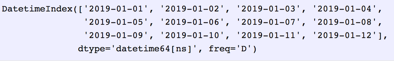
Let’s say we need a date range incremented by days.
date_from = "2019-01-01"
date_to = "2019-01-12"
date_range = pd.date_range(date_from, date_to, freq="D")
date_range

Let’s transform the generated date_range to start and end dates, which can be passed to a subsequent function.
for i, (date_from, date_to) in enumerate(zip(date_range[:-1], date_range[1:]), 1):
    date_from = date_from.date().isoformat()
    date_to = date_to.date().isoformat()
    print("%d. date_from: %s, date_to: %s" % (i, date_from, date_to))1. date_from: 2019-01-01, date_to: 2019-01-02
2. date_from: 2019-01-02, date_to: 2019-01-03
3. date_from: 2019-01-03, date_to: 2019-01-04
4. date_from: 2019-01-04, date_to: 2019-01-05
5. date_from: 2019-01-05, date_to: 2019-01-06
6. date_from: 2019-01-06, date_to: 2019-01-07
7. date_from: 2019-01-07, date_to: 2019-01-08
8. date_from: 2019-01-08, date_to: 2019-01-09
9. date_from: 2019-01-09, date_to: 2019-01-10
10. date_from: 2019-01-10, date_to: 2019-01-11
11. date_from: 2019-01-11, date_to: 2019-01-12
2. Merge with indicator
Merging
two datasets is the process of bringing two datasets together into one,
and aligning the rows from each based on common attributes or columns.
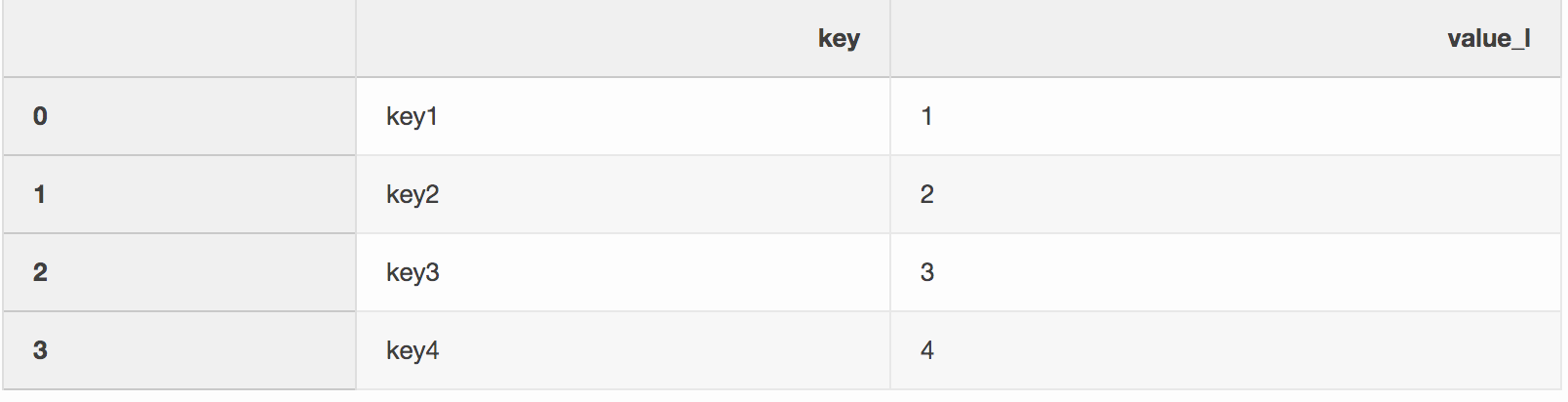
One of the arguments of the merge function that I’ve missed is the
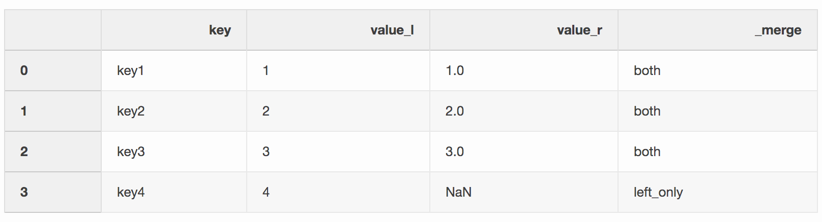
indicator argument. Indicator argument adds a _merge column to a DataFrame, which tells you “where the row came from”, left, right or both DataFrames. The _merge column can be very useful when working with bigger datasets to check the correctness of a merge operation.left = pd.DataFrame({"key": ["key1", "key2", "key3", "key4"], "value_l": [1, 2, 3, 4]})

right = pd.DataFrame({"key": ["key3", "key2", "key1", "key6"], "value_r": [3, 2, 1, 6]})
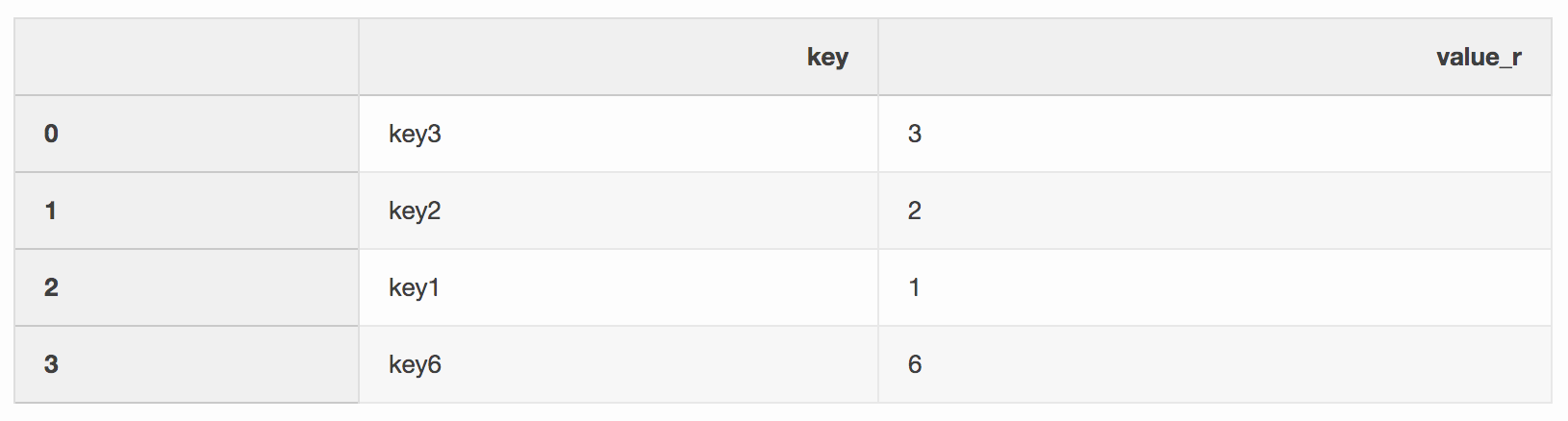
df_merge = left.merge(right, on='key', how='left', indicator=True)
The
_merge column can be used to check if there is an expected number of rows with values from both DataFrames.df_merge._merge.value_counts()both 3 left_only 1 right_only 0 Name: _merge, dtype: int64
3. Nearest merge
When
working with financial data, like stocks or cryptocurrencies, we may
need to combine quotes (price changes) with actual trades. Let’s say
that we would like to merge each trade with a quote that occurred a few
milliseconds before it. Pandas has a function merge_asof, which enables
merging DataFrames by the nearest key (timestamp in our example). The
datasets quotes and trades are taken from pandas example
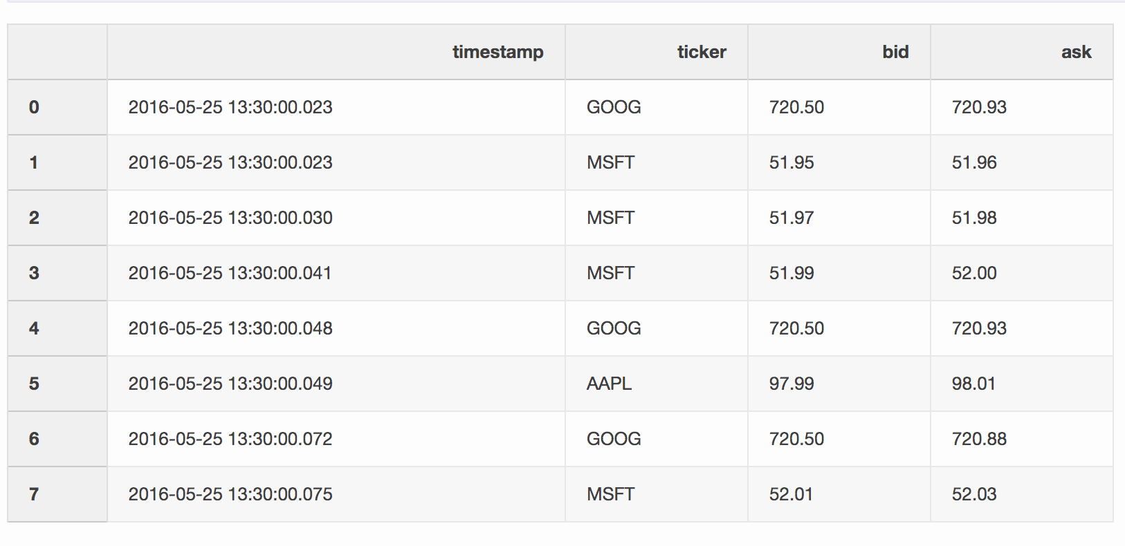
The quotes DataFrame contains price changes for different stocks. Usually, there are many more quotes than trades.
quotes = pd.DataFrame(
    [
        ["2016-05-25 13:30:00.023", "GOOG", 720.50, 720.93],
        ["2016-05-25 13:30:00.023", "MSFT", 51.95, 51.96],
        ["2016-05-25 13:30:00.030", "MSFT", 51.97, 51.98],
        ["2016-05-25 13:30:00.041", "MSFT", 51.99, 52.00],
        ["2016-05-25 13:30:00.048", "GOOG", 720.50, 720.93],
        ["2016-05-25 13:30:00.049", "AAPL", 97.99, 98.01],
        ["2016-05-25 13:30:00.072", "GOOG", 720.50, 720.88],
        ["2016-05-25 13:30:00.075", "MSFT", 52.01, 52.03],
    ],
    columns=["timestamp", "ticker", "bid", "ask"],
)
quotes['timestamp'] = pd.to_datetime(quotes['timestamp'])

The trades DataFrame contains trades of different stocks.
trades = pd.DataFrame(
    [
        ["2016-05-25 13:30:00.023", "MSFT", 51.95, 75],
        ["2016-05-25 13:30:00.038", "MSFT", 51.95, 155],
        ["2016-05-25 13:30:00.048", "GOOG", 720.77, 100],
        ["2016-05-25 13:30:00.048", "GOOG", 720.92, 100],
        ["2016-05-25 13:30:00.048", "AAPL", 98.00, 100],
    ],
    columns=["timestamp", "ticker", "price", "quantity"],
)
trades['timestamp'] = pd.to_datetime(trades['timestamp'])

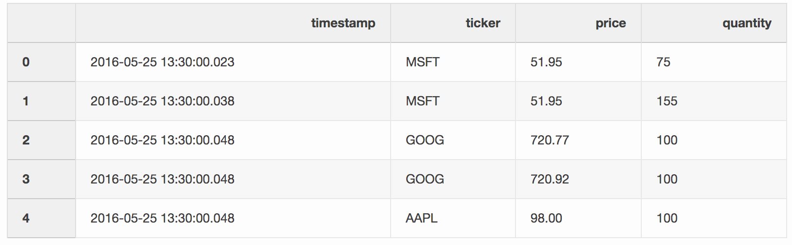
We
merge trades and quotes by tickers, where the latest quote can be 10 ms
behind the trade. If a quote is more than 10 ms behind the trade or
there isn’t any quote, the bid and ask for that quote will be null (AAPL
ticker in this example).
pd.merge_asof(trades, quotes, on="timestamp", by='ticker', tolerance=pd.Timedelta('10ms'), direction='backward')


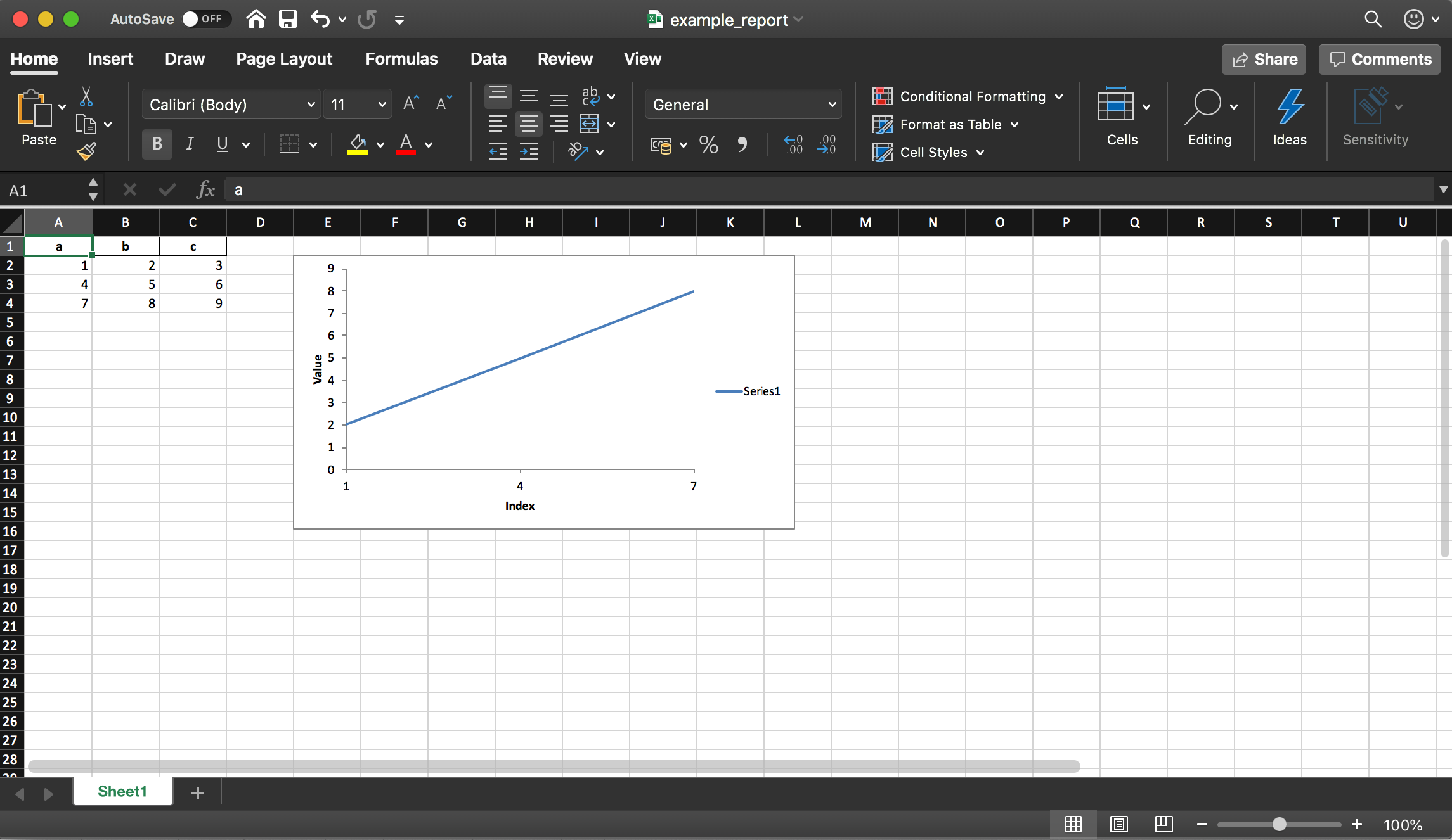
4. Create an Excel report

Pandas
(with XlsxWriter library) enables us to create an Excel report from the
DataFrame. This is a major time saver — no more saving a DataFrame to
CSV and then formatting it in Excel. We can also add all kinds of charts, etc.
df = pd.DataFrame(pd.np.array([[1, 2, 3], [4, 5, 6], [7, 8, 9]]), columns=["a", "b", "c"])
The code snippet below creates an Excel report. To save a DataFrame to the Excel file, uncomment the
writer.save() line.report_name = 'example_report.xlsx' sheet_name = 'Sheet1'writer = pd.ExcelWriter(report_name, engine='xlsxwriter') df.to_excel(writer, sheet_name=sheet_name, index=False) # writer.save()
As
mentioned before, the library also supports adding charts to the Excel
report. We need to define the type of the chart (line chart in our
example) and the data series for the chart (the data series needs to be
in the Excel spreadsheet).
# define the workbookworkbook = writer.book
worksheet = writer.sheets[sheet_name]# create a chart line objectchart = workbook.add_chart({'type': 'line'})# configure the series of the chart from the spreadsheet
# using a list of values instead of category/value formulas:
#     [sheetname, first_row, first_col, last_row, last_col]chart.add_series({
    'categories': [sheet_name, 1, 0, 3, 0],
    'values':     [sheet_name, 1, 1, 3, 1],
})# configure the chart axeschart.set_x_axis({'name': 'Index', 'position_axis': 'on_tick'})
chart.set_y_axis({'name': 'Value', 'major_gridlines': {'visible': False}})# place the chart on the worksheetworksheet.insert_chart('E2', chart)# output the excel filewriter.save()
5. Save the disk space
When
working on multiple Data Science projects, you usually end up with many
preprocessed datasets from different experiments. Your SSD on a laptop
can get cluttered quickly. Pandas enables you to compress the dataset
when saving it and then reading back in compressed format.
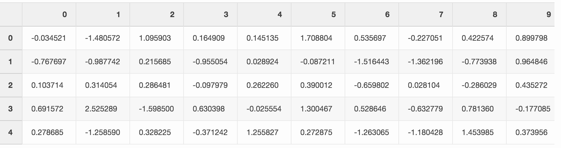
Let’s create a big pandas DataFrame with random numbers.
df = pd.DataFrame(pd.np.random.randn(50000,300))

When we save this file as CSV, it takes almost 300 MB on the hard drive.
df.to_csv('random_data.csv', index=False)
With a single argument
compression='gzip', we can reduce the file size to 136 MB.df.to_csv('random_data.gz', compression='gzip', index=False)
It is also easy to read the gzipped data to the DataFrame, so we don’t lose any functionality.
df = pd.read_csv('random_data.gz')
Conclusion
These
tricks help me daily to be more productive with pandas. Hopefully, this
blog post showed you a new pandas function, that will help you to be
more productive.
What’s your favorite pandas trick?
Pure Salon & Spa Koramangla, Bangalore
Led by veteran hair stylist Pure Salon & Spa offers various services from the simple hair cut and styling for women, men, kids, and brides, to vibrant hair colours, conditioning treatments, and Brazilian blowouts. Located at the heart of Koramangla, Bangalore, the salon has been around since 2015, providing professional hair treatments in a relaxed ambience. This is definitely one of our favourite hair salons in Bangalore.
Cape Clean - India's Top Facade and Window Cleaning